Stop-Limit Order Execution via Martingale Theory

In financial markets, traders routinely face the challenge of optimizing entry and exit points in an environment characterized by uncertainty. This article examines the mathematical foundations of stop-limit orders—a powerful trading mechanism that combines protective stops with opportunistic limits—through the lens of stochastic calculus. By modeling asset price movements as a geometric Brownian motion, we derive an elegant formula for the probability that a limit order will execute before a stop order is triggered.

Stops vs Limits: The Fundamentals

A stop order is an instruction to trade when the price of a market hits a specific level that is less favourable than the current price. On the other hand, a limit order is an instruction to trade if the market price reaches a specified level more favourable than the current price.

There is no reason to only use one or the other type of order – both are extremely useful tools for a trader. In fact, some platforms go so far as to combine both orders into a single ‘stop-limit order’. This would enable traders to predefine their conditions for trading, entering a trend at a certain price level and exiting the trade once they’ve taken a certain amount of profit. Therefore, if we can understand the probability of a stop order getting triggered as opposed to a limit order, we can then estimate the expected return of a single stop-limit order.

Modeling Price Movements with Geometric Brownian Motion

To analyze these probabilities mathematically, we'll model stock price movements using a geometric Brownian motion (GBM). This is a continuous-time stochastic process where the logarithm of the randomly varying quantity follows a Brownian motion with drift.

A stock price $S_t$ follows a GBM if it satisfies the following stochastic differential equation:

$$dS_t = \mu S_t dt + \sigma S_t dW_t$$

where:

• $W_t$ represents a Wiener process (standard Brownian motion)
• $\mu$ is the expected return (drift coefficient)
• $\sigma$ is the volatility (standard deviation of returns)

For any initial value $S_0$, this SDE has the analytical solution:

$$S_t = S_0 \exp \left[ \left( \mu - \frac{\sigma^2}{2} \right) t + \sigma W_t \right]$$

This equation gives us the stock price at any future time $t$ based on the initial price and the parameters of the process.

The Two-Boundary Problem

In the context of stop-limit orders, we're interested in the first passage time problem with two absorbing boundaries. Let's define:

• $\alpha$ as the upper boundary (limit price)
• $\beta$ as the lower boundary (stop price)
• $S_0$ as the current stock price, with $\alpha > S_0 > \beta$

We want to determine the probability that the stock price $S_t$ will hit the upper boundary $\alpha$ at time $t = \tau_\alpha$ without ever hitting the lower boundary $\beta$. This would represent the probability of a limit order executing before a stop order.

Applying the Optional Stopping Theorem

The optional stopping theorem from probability theory states that a martingale stopped at a stopping time remains a martingale. This means the expected value of a martingale at a stopping time equals its initial expected value.

We'll use the exponential martingale, which has the form:

$$Z_t = \exp \left[ \lambda W_t - \frac{1}{2} \lambda^2 t \right]$$

This is a martingale for any value of $\lambda$, which we'll use to our advantage.

Transformation of Variables

To simplify our analysis, let's transform the stock price process into a more manageable form. We define a new variable $Y_t$ as:

$$Y_t = \frac{\log (S_t) - \log (S_0)}{\sigma}$$

Substituting the expression for $S_t$, we get:

$$\begin{aligned} Y_t &= \frac{\log \left( S_0 \exp \left[ \left( \mu - \frac{\sigma^2}{2} \right) t + \sigma W_t \right] \right) - \log (S_0)}{\sigma} \\ &= \left( \frac{\mu}{\sigma} - \frac{\sigma}{2} \right) t + W_t \\ &= \tilde{\mu} t + W_t \end{aligned}$$

where we've defined $\tilde{\mu} = \frac{\mu}{\sigma} - \frac{\sigma}{2}$ for convenience.

Creating a Time-Independent Martingale

Now we can express $W_t$ in terms of $Y_t$:

$$W_t = Y_t - \tilde{\mu} t$$

Substituting this into our exponential martingale:

$$\begin{aligned} Z_t &= \exp \left[ \lambda W_t - \frac{1}{2} \lambda^2 t \right] \\ &= \exp \left[ \lambda (Y_t - \tilde{\mu} t) - \frac{1}{2} \lambda^2 t \right] \\ &= \exp \left[ \lambda Y_t - t\left(\lambda\tilde{\mu} + \frac{1}{2} \lambda^2\right) \right] \end{aligned}$$

To eliminate the time-dependent term, we need:

$$\lambda\tilde{\mu} + \frac{1}{2} \lambda^2 = 0$$

Solving for $\lambda$:

$$\lambda = 0 \text{ or } \lambda = -2\tilde{\mu}$$

We choose $\lambda = -2\tilde{\mu}$ (the non-trivial solution), which gives us:

$$Z_t = \exp \left( -2 \tilde{\mu} Y_t \right)$$

This is now a time-independent martingale.

Finding the Probability

Let $p_\alpha$ be the probability that the process hits the upper boundary $\alpha$ before hitting the lower boundary $\beta$.

At the stopping time $\tau = \min(\tau_\alpha, \tau_\beta)$, the process will be at either boundary:

• With probability $p_\alpha$, it hits $\alpha$ first, and $Y_{\tau} = Y_{\tau_\alpha} = \frac{\log \alpha - \log S_0}{\sigma}$
• With probability $1-p_\alpha$, it hits $\beta$ first, and $Y_{\tau} = Y_{\tau_\beta} = \frac{\log \beta - \log S_0}{\sigma}$

By the optional stopping theorem, we know that $\mathbb{E}[Z_\tau] = \mathbb{E}[Z_0] = 1$.

Therefore:

$$\begin{aligned} \mathbb{E}[Z_\tau] &= p_\alpha \cdot \exp(-2\tilde{\mu}Y_{\tau_\alpha}) + (1-p_\alpha) \cdot \exp(-2\tilde{\mu}Y_{\tau_\beta}) \\ &= p_\alpha \cdot \exp\left(-2\tilde{\mu}\frac{\log \alpha - \log S_0}{\sigma}\right) + (1-p_\alpha) \cdot \exp\left(-2\tilde{\mu}\frac{\log \beta - \log S_0}{\sigma}\right) \\ &= 1 \end{aligned}$$

Solving for $p_\alpha$ gives us our final result:

$$p_\alpha = \frac{1 - \exp(-2\tilde{\mu}Y_{\tau_\beta})}{\exp(-2\tilde{\mu}Y_{\tau_\alpha}) - \exp(-2\tilde{\mu}Y_{\tau_\beta})}$$

This formula gives us the probability that a limit order at price $\alpha$ will be executed before a stop order at price $\beta$, assuming the stock price follows a geometric Brownian motion with drift $\mu$ and volatility $\sigma$.

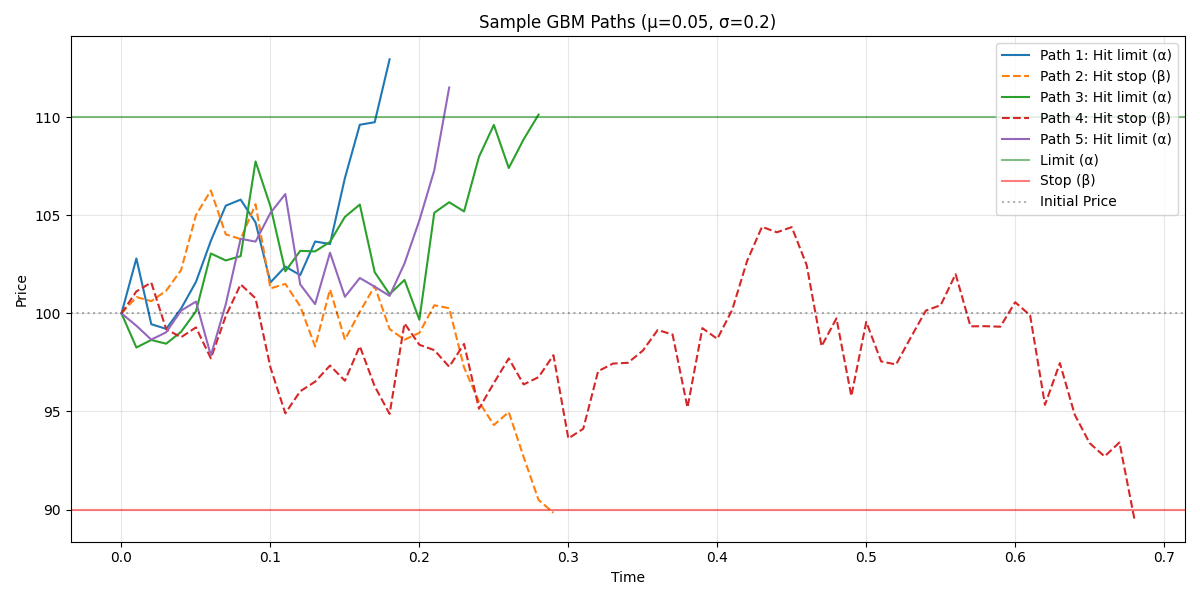
Monte Carlo Simulations

We can simulate financial asset price movements using Geometric Brownian Motion (GBM) with absorbing boundaries, calculating both theoretical probabilities and empirical results from Monte Carlo simulations. The methodology tests how drift parameters, volatility values, and boundary configurations affect the probability of hitting upper boundaries before lower ones, validating theoretical formulas with empirical tests across 10,000 simulation paths per parameter combination. The code is available at my GitHub repository.

Results Summary

Parameter Type	Parameter Values	Theoretical Probability	Empirical Probability	Absolute Error	Relative Error (%)
Drift (μ)	μ = -0.10, σ = 0.2	0.3778	0.3688	0.0090	2.39
	μ = -0.05, σ = 0.2	0.4378	0.4332	0.0046	1.06
	μ = 0.00, σ = 0.2	0.5000	0.4944	0.0056	1.12
	μ = 0.05, σ = 0.2	0.5624	0.5626	0.0002	0.03
	μ = 0.10, σ = 0.2	0.6231	0.6261	0.0030	0.47
Volatility (σ)	μ = 0.05, σ = 0.1	0.7330	0.7306	0.0024	0.33
	μ = 0.05, σ = 0.2	0.5624	0.5587	0.0037	0.66
	μ = 0.05, σ = 0.3	0.5278	0.5291	0.0013	0.24
	μ = 0.05, σ = 0.4	0.5157	0.5045	0.0112	2.16
Boundaries	S₀ = 100, α = 105, β = 95	0.5312	0.5314	0.0002	0.03
	S₀ = 100, α = 110, β = 90	0.5624	0.5619	0.0005	0.09
	S₀ = 100, α = 120, β = 80	0.6243	0.6212	0.0031	0.49
	S₀ = 100, α = 120, β = 90	0.4171	0.4209	0.0038	0.91
	S₀ = 100, α = 110, β = 80	0.7490	0.7428	0.0062	0.83

Key Insights

The simulations validate the theoretical framework with excellent accuracy, achieving relative errors typically below 1%. Three fundamental patterns emerge from the analysis:

Drift acts as a directional bias: positive drift increases the probability of hitting upper boundaries, with the effect being roughly linear—each increment in drift shifts probabilities by several percentage points in the expected direction.

Volatility diminishes drift effects: higher volatility causes the process to behave more randomly, reducing the influence of drift and pushing probabilities toward 50/50 regardless of directional bias. This explains why low-volatility assets exhibit more predictable directional behavior.

Boundary asymmetry matters significantly: the relative distances of boundaries from the starting price are critical. Moving one boundary farther away substantially increases the probability of hitting the opposite boundary first, demonstrating that stop-limit order placement requires careful consideration of both absolute and relative positioning.